Difference between revisions of "Directory:Jon Awbrey/Papers/Differential Logic : Introduction"
Jon Awbrey (talk | contribs) (→Operational Representation: + next paragraph) |
Jon Awbrey (talk | contribs) (→Operational Representation: + next sentence) |
||
| Line 1,046: | Line 1,046: | ||
It happens that there are just two possible groups of 4 elements. One is the cyclic group <math>Z_4\!</math> (from German ''Zyklus''), which this is not. The other is the Klein four-group <math>V_4\!</math> (from German ''Vier''), which this is. | It happens that there are just two possible groups of 4 elements. One is the cyclic group <math>Z_4\!</math> (from German ''Zyklus''), which this is not. The other is the Klein four-group <math>V_4\!</math> (from German ''Vier''), which this is. | ||
| + | |||
| + | More concretely viewed, the group as a whole pushes the set of sixteen propositions around in such a way that they fall into seven natural classes, called ''orbits''. One says that the orbits are preserved by the action of the group. There is an ''Orbit Lemma'' of immense utility to “those who count” which, depending on your upbringing, you may associate with the names of Burnside, Cauchy, Frobenius, or some subset or superset of these three, vouching that the number of orbits is equal to the mean number of fixed points, in other words, the total number of points (in our case, propositions) that are left unmoved by the separate operations, divided by the order of the group. | ||
==Propositional Forms on Two Variables== | ==Propositional Forms on Two Variables== | ||
Revision as of 18:42, 30 November 2015
- Note. The MathJax parser is not rendering this page properly.
Until it can be fixed please see the InterSciWiki version.
Author: Jon Awbrey
Differential logic is the component of logic whose object is the description of variation — for example, the aspects of change, difference, distribution, and diversity — in universes of discourse that are subject to logical description. A definition that broad naturally incorporates any study of variation by way of mathematical models, but differential logic is especially charged with the qualitative aspects of variation that pervade or precede quantitative models. To the extent that a logical inquiry makes use of a formal system, its differential component treats the principles that govern the use of a differential logical calculus, that is, a formal system with the expressive capacity to describe change and diversity in a logical universe of discourse.
A simple example of a differential logical calculus is furnished by a differential propositional calculus. A differential propositional calculus is a propositional calculus extended by a set of terms for describing aspects of change and difference, for example, processes that take place in a universe of discourse or transformations that map a source universe into a target universe. This augments ordinary propositional calculus in the same way that the differential calculus of Leibniz and Newton augments the analytic geometry of Descartes.
Quick Overview
Cactus Language for Propositional Logic
The development of differential logic is greatly facilitated by having a conceptually efficient calculus in place at the level of boolean-valued functions and elementary logical propositions. A calculus that is very efficient from both conceptual and computational standpoints is based on just two types of logical connectives, both of variable \(k\!\)-ary scope. The formulas of this calculus map into a species of graph-theoretical structures called painted and rooted cacti (PARCs) that lend visual representation to their functional structure and smooth the path to efficient computation.
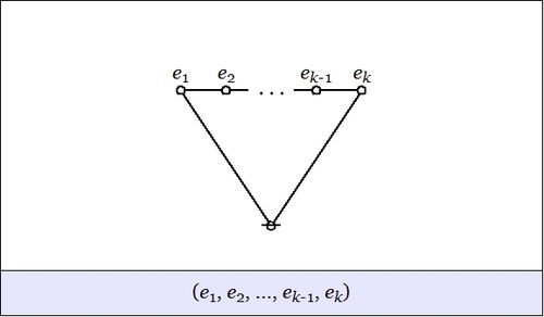
| The first kind of propositional expression is a parenthesized sequence of propositional expressions, written as \(\texttt{(} e_1 \texttt{,} e_2 \texttt{,} \ldots \texttt{,} e_{k-1} \texttt{,} e_k \texttt{)}\!\) and read to say that exactly one of the propositions \(e_1, e_2, \ldots, e_{k-1}, e_k\!\) is false, in other words, that their minimal negation is true. A clause of this form maps into a PARC structure called a lobe, in this case, one that is painted with the colors \(e_1, e_2, \ldots, e_{k-1}, e_k\!\) as shown below. |
|
| The second kind of propositional expression is a concatenated sequence of propositional expressions, written as \(e_1\ e_2\ \ldots\ e_{k-1}\ e_k\!\) and read to say that all of the propositions \(e_1, e_2, \ldots, e_{k-1}, e_k\!\) are true, in other words, that their logical conjunction is true. A clause of this form maps into a PARC structure called a node, in this case, one that is painted with the colors \(e_1, e_2, \ldots, e_{k-1}, e_k\!\) as shown below. |

|
All other propositional connectives can be obtained through combinations of these two forms. Strictly speaking, the parenthesized form is sufficient to define the concatenated form, making the latter formally dispensable, but it is convenient to maintain it as a concise way of expressing more complicated combinations of parenthesized forms. While working with expressions solely in propositional calculus, it is easiest to use plain parentheses for logical connectives. In contexts where ordinary parentheses are needed for other purposes an alternate typeface \(\texttt{(} \ldots \texttt{)}\!\) may be used for logical operators.
Table 1 collects a sample of basic propositional forms as expressed in terms of cactus language connectives.
The simplest expression for logical truth is the empty word, usually denoted by \(\boldsymbol\varepsilon\!\) or \(\lambda\!\) in formal languages, where it forms the identity element for concatenation. To make it visible in context, it may be denoted by the equivalent expression \({}^{\backprime\backprime} \texttt{((~))} {}^{\prime\prime},\!\) or, especially if operating in an algebraic context, by a simple \({}^{\backprime\backprime} 1 {}^{\prime\prime}.\!\) Also when working in an algebraic mode, the plus sign \({}^{\backprime\backprime} + {}^{\prime\prime}\!\) may be used for exclusive disjunction. For example, we have the following paraphrases of algebraic expressions by means of parenthesized expressions:
|
\(\begin{matrix} a + b & = & \texttt{(} a \texttt{,} b \texttt{)} \end{matrix}\!\) |
|
\(\begin{matrix} a + b + c & = & \texttt{(} a \texttt{,(} b \texttt{,} c \texttt{))} & = & \texttt{((} a \texttt{,} b \texttt{),} c \texttt{)} \end{matrix}\!\) |
It is important to note that the last expressions are not equivalent to the 3-place parenthesis \(\texttt{(} a \texttt{,} b \texttt{,} c \texttt{)}.\!\)
Differential Expansions of Propositions
Bird's Eye View
An efficient calculus for the realm of logic represented by boolean functions and elementary propositions makes it feasible to compute the finite differences and the differentials of those functions and propositions.
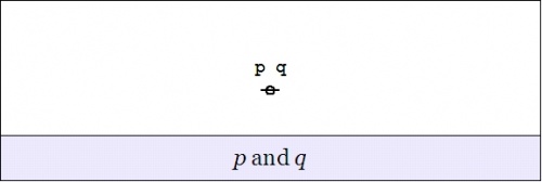
For example, consider a proposition of the form \({}^{\backprime\backprime} \, p ~\mathrm{and}~ q \, {}^{\prime\prime}\!\) that is graphed as two letters attached to a root node:
|
Written as a string, this is just the concatenation \(p~q\!\).
The proposition \(pq\!\) may be taken as a boolean function \(f(p, q)\!\) having the abstract type \(f : \mathbb{B} \times \mathbb{B} \to \mathbb{B},\!\) where \(\mathbb{B} = \{ 0, 1 \}~\!\) is read in such a way that \(0\!\) means \(\mathrm{false}\!\) and \(1\!\) means \(\mathrm{true}.\!\)
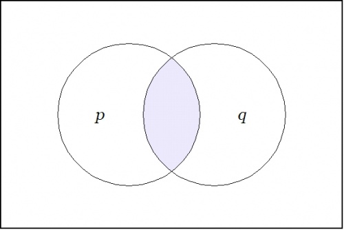
Imagine yourself standing in a fixed cell of the corresponding venn diagram, say, the cell where the proposition \(pq\!\) is true, as shown in the following Figure:
|
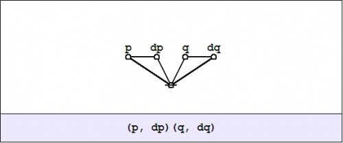
Now ask yourself: What is the value of the proposition \(pq\!\) at a distance of \(\mathrm{d}p\!\) and \(\mathrm{d}q\!\) from the cell \(pq\!\) where you are standing?
Don't think about it — just compute:
|
The cactus formula \(\texttt{(p, dp)(q, dq)}\!\) and its corresponding graph arise by substituting \(p + \mathrm{d}p\!\) for \(p\!\) and \(q + \mathrm{d}q\!\) for \(q\!\) in the boolean product or logical conjunction \(pq\!\) and writing the result in the two dialects of cactus syntax. This follows from the fact that the boolean sum \(p + \mathrm{d}p\!\) is equivalent to the logical operation of exclusive disjunction, which parses to a cactus graph of the following form:
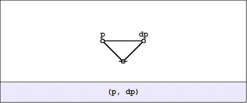
|
Next question: What is the difference between the value of the proposition \(pq\!\) over there, at a distance of \(\mathrm{d}p\!\) and \(\mathrm{d}q,\!\) and the value of the proposition \(pq\!\) where you are standing, all expressed in the form of a general formula, of course? Here is the appropriate formulation:
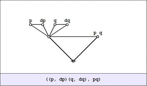
|
There is one thing that I ought to mention at this point: Computed over \(\mathbb{B},\!\) plus and minus are identical operations. This will make the relation between the differential and the integral parts of the appropriate calculus slightly stranger than usual, but we will get into that later.
Last question, for now: What is the value of this expression from your current standpoint, that is, evaluated at the point where \(pq\!\) is true? Well, substituting \(1\!\) for \(p\!\) and \(1\!\) for \(q\!\) in the graph amounts to erasing the labels \(p\!\) and \(q\!,\!\) as shown here:
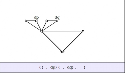
|
And this is equivalent to the following graph:
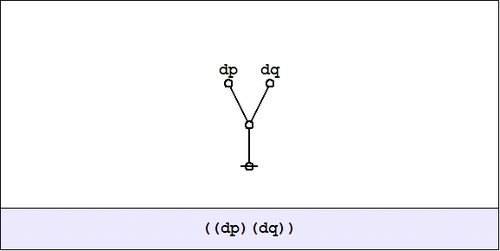
|
We have just met with the fact that the differential of the and is the or of the differentials.
|
\(\begin{matrix} p ~\mathrm{and}~ q & \quad & \xrightarrow{\quad\mathrm{Diff}\quad} & \quad & \mathrm{d}p ~\mathrm{or}~ \mathrm{d}q \end{matrix}\!\) |
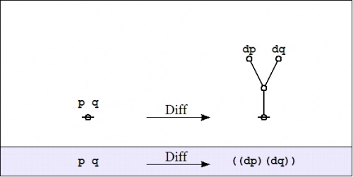
|
It will be necessary to develop a more refined analysis of that statement directly, but that is roughly the nub of it.
If the form of the above statement reminds you of De Morgan's rule, it is no accident, as differentiation and negation turn out to be closely related operations. Indeed, one can find discussions of logical difference calculus in the Boole–De Morgan correspondence and Peirce also made use of differential operators in a logical context, but the exploration of these ideas has been hampered by a number of factors, not the least of which has been the lack of a syntax that was adequate to handle the complexity of expressions that evolve.
Worm's Eye View
Let's run through the initial example again, this time attempting to interpret the formulas that develop at each stage along the way. We begin with a proposition or a boolean function \(f(p, q) = pq.\!\)

|

|
A function like this has an abstract type and a concrete type. The abstract type is what we invoke when we write things like \(f : \mathbb{B} \times \mathbb{B} \to \mathbb{B}\!\) or \(f : \mathbb{B}^2 \to \mathbb{B}.\!\) The concrete type takes into account the qualitative dimensions or the “units” of the case, which can be explained as follows.
| Let \(P\!\) be the set of values \(\{ \texttt{(} p \texttt{)},~ p \} ~=~ \{ \mathrm{not}~ p,~ p \} ~\cong~ \mathbb{B}.\!\) |
| Let \(Q\!\) be the set of values \(\{ \texttt{(} q \texttt{)},~ q \} ~=~ \{ \mathrm{not}~ q,~ q \} ~\cong~ \mathbb{B}.\!\) |
Then interpret the usual propositions about \(p, q\!\) as functions of the concrete type \(f : P \times Q \to \mathbb{B}.\!\)
We are going to consider various operators on these functions. Here, an operator \(\mathrm{F}\!\) is a function that takes one function \(f\!\) into another function \(\mathrm{F}f.\!\)
The first couple of operators that we need to consider are logical analogues of the pair that play a founding role in the classical finite difference calculus, namely:
| The difference operator \(\Delta,\!\) written here as \(\mathrm{D}.\!\) |
| The enlargement operator \(\Epsilon,\!\) written here as \(\mathrm{E}.\!\) |
These days, \(\mathrm{E}\!\) is more often called the shift operator.
In order to describe the universe in which these operators operate, it is necessary to enlarge the original universe of discourse. Starting from the initial space \(X = P \times Q,\!\) its (first order) differential extension \(\mathrm{E}X\!\) is constructed according to the following specifications:
|
\(\begin{array}{rcc} \mathrm{E}X & = & X \times \mathrm{d}X \end{array}\!\) |
where:
|
\(\begin{array}{rcc} X & = & P \times Q \\[4pt] \mathrm{d}X & = & \mathrm{d}P \times \mathrm{d}Q \\[4pt] \mathrm{d}P & = & \{ \texttt{(} \mathrm{d}p \texttt{)},~ \mathrm{d}p \} \\[4pt] \mathrm{d}Q & = & \{ \texttt{(} \mathrm{d}q \texttt{)},~ \mathrm{d}q \} \end{array}\!\) |
The interpretations of these new symbols can be diverse, but the easiest option for now is just to say that \(\mathrm{d}p\!\) means “change \(p\!\)” and \(\mathrm{d}q\!\) means “change \(q\!\)”.
Drawing a venn diagram for the differential extension \(\mathrm{E}X = X \times \mathrm{d}X\!\) requires four logical dimensions, \(P, Q, \mathrm{d}P, \mathrm{d}Q,\!\) but it is possible to project a suggestion of what the differential features \(\mathrm{d}p\!\) and \(\mathrm{d}q\!\) are about on the 2-dimensional base space \(X = P \times Q\!\) by drawing arrows that cross the boundaries of the basic circles in the venn diagram for \(X,\!\) reading an arrow as \(\mathrm{d}p\!\) if it crosses the boundary between \(p\!\) and \(\texttt{(} p \texttt{)}\!\) in either direction and reading an arrow as \(\mathrm{d}q\!\) if it crosses the boundary between \(q\!\) and \(\texttt{(} q \texttt{)}\!\) in either direction.

|
Propositions are formed on differential variables, or any combination of ordinary logical variables and differential logical variables, in the same ways that propositions are formed on ordinary logical variables alone. For example, the proposition \(\texttt{(} \mathrm{d}p \texttt{(} \mathrm{d}q \texttt{))}\!\) says the same thing as \(\mathrm{d}p \Rightarrow \mathrm{d}q,\!\) in other words, that there is no change in \(p\!\) without a change in \(q.\!\)
Given the proposition \(f(p, q)\!\) over the space \(X = P \times Q,\!\) the (first order) enlargement of \(f\!\) is the proposition \(\mathrm{E}f\!\) over the differential extension \(\mathrm{E}X\!\) that is defined by the following formula:
|
\(\begin{matrix} \mathrm{E}f(p, q, \mathrm{d}p, \mathrm{d}q) & = & f(p + \mathrm{d}p,~ q + \mathrm{d}q) & = & f( \texttt{(} p, \mathrm{d}p \texttt{)},~ \texttt{(} q, \mathrm{d}q \texttt{)} ) \end{matrix}\!\) |
In the example \(f(p, q) = pq,\!\) the enlargement \(\mathrm{E}f\!\) is computed as follows:
|
\(\begin{matrix} \mathrm{E}f(p, q, \mathrm{d}p, \mathrm{d}q) & = & (p + \mathrm{d}p)(q + \mathrm{d}q) & = & \texttt{(} p, \mathrm{d}p \texttt{)(} q, \mathrm{d}q \texttt{)} \end{matrix}\!\) |
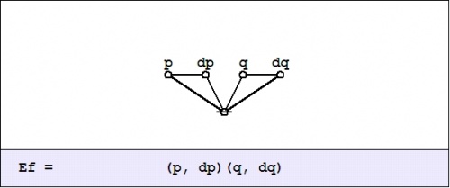
|
Given the proposition \(f(p, q)\!\) over \(X = P \times Q,\!\) the (first order) difference of \(f\!\) is the proposition \(\mathrm{D}f~\!\) over \(\mathrm{E}X\!\) that is defined by the formula \(\mathrm{D}f = \mathrm{E}f - f,\!\) or, written out in full:
|
\(\begin{matrix} \mathrm{D}f(p, q, \mathrm{d}p, \mathrm{d}q) & = & f(p + \mathrm{d}p,~ q + \mathrm{d}q) - f(p, q) & = & \texttt{(} f( \texttt{(} p, \mathrm{d}p \texttt{)},~ \texttt{(} q, \mathrm{d}q \texttt{)} ),~ f(p, q) \texttt{)} \end{matrix}\!\) |
In the example \(f(p, q) = pq,\!\) the difference \(\mathrm{D}f~\!\) is computed as follows:
We did not yet go through the trouble to interpret this (first order) difference of conjunction fully, but were happy simply to evaluate it with respect to a single location in the universe of discourse, namely, at the point picked out by the singular proposition \(pq,\!\) that is, at the place where \(p = 1\!\) and \(q = 1.\!\) This evaluation is written in the form \(\mathrm{D}f|_{pq}\!\) or \(\mathrm{D}f|_{(1, 1)},\!\) and we arrived at the locally applicable law that is stated and illustrated as follows:
|
\(f(p, q) ~=~ pq ~=~ p ~\mathrm{and}~ q \quad \Rightarrow \quad \mathrm{D}f|_{pq} ~=~ \texttt{((} \mathrm{dp} \texttt{)(} \mathrm{d}q \texttt{))} ~=~ \mathrm{d}p ~\mathrm{or}~ \mathrm{d}q\!\) |

|

|
The picture shows the analysis of the inclusive disjunction \(\texttt{((} \mathrm{d}p \texttt{)(} \mathrm{d}q \texttt{))}\!\) into the following exclusive disjunction:
|
\(\begin{matrix} \mathrm{d}p ~\texttt{(} \mathrm{d}q \texttt{)} & + & \texttt{(} \mathrm{d}p \texttt{)}~ \mathrm{d}q & + & \mathrm{d}p ~\mathrm{d}q \end{matrix}\!\) |
The differential proposition that results may be interpreted to say “change \(p\!\) or change \(q\!\) or both”. And this can be recognized as just what you need to do if you happen to find yourself in the center cell and require a complete and detailed description of ways to escape it.
Last time we computed what is variously called the difference map, the difference proposition, or the local proposition \(\mathrm{D}f_x\!\) of the proposition \(f(p, q) = pq\!\) at the point \(x\!\) where \(p = 1\!\) and \(q = 1.\!\)
In the universe \(X = P \times Q,\!\) the four propositions \(pq,~ p \texttt{(} q \texttt{)},~ \texttt{(} p \texttt{)} q,~ \texttt{(} p \texttt{)(} q \texttt{)}\!\) that indicate the “cells”, or the smallest regions of the venn diagram, are called singular propositions. These serve as an alternative notation for naming the points \((1, 1),~ (1, 0),~ (0, 1),~ (0, 0),\!\) respectively.
Thus we can write \(\mathrm{D}f_x = \mathrm{D}f|x = \mathrm{D}f|(1, 1) = \mathrm{D}f|pq,\!\) so long as we know the frame of reference in force.
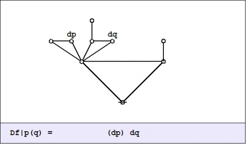
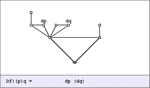
In the example \(f(p, q) = pq,\!\) the value of the difference proposition \(\mathrm{D}f_x\!\) at each of the four points in \(x \in X\!\) may be computed in graphical fashion as shown below:
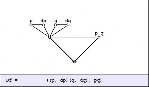
|
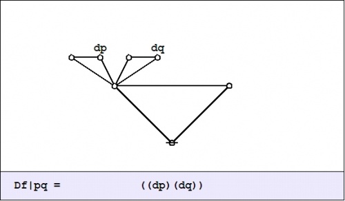
|
|
|

|
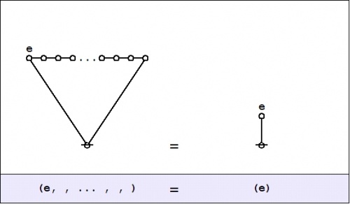
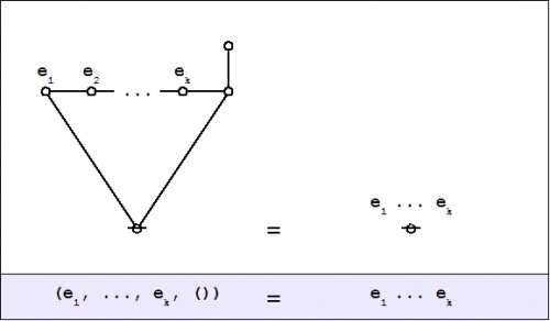
The easy way to visualize the values of these graphical expressions is just to notice the following equivalents:
|
|
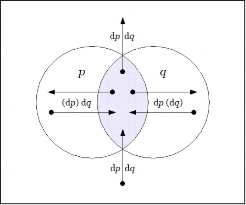
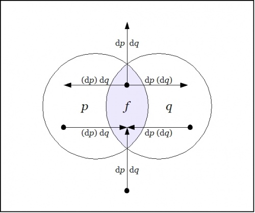
Laying out the arrows on the augmented venn diagram, one gets a picture of a differential vector field.
|
The Figure shows the points of the extended universe \(\mathrm{E}X = P \times Q \times \mathrm{d}P \times \mathrm{d}Q\!\) that are indicated by the difference map \(\mathrm{D}f : \mathrm{E}X \to \mathbb{B},\!\) namely, the following six points or singular propositions::
|
\(\begin{array}{rcccc} 1. & p & q & \mathrm{d}p & \mathrm{d}q \\ 2. & p & q & \mathrm{d}p & (\mathrm{d}q) \\ 3. & p & q & (\mathrm{d}p) & \mathrm{d}q \\ 4. & p & (q) & (\mathrm{d}p) & \mathrm{d}q \\ 5. & (p) & q & \mathrm{d}p & (\mathrm{d}q) \\ 6. & (p) & (q) & \mathrm{d}p & \mathrm{d}q \end{array}\!\) |
The information borne by \(\mathrm{D}f~\!\) should be clear enough from a survey of these six points — they tell you what you have to do from each point of \(X\!\) in order to change the value borne by \(f(p, q),\!\) that is, the move you have to make in order to reach a point where the value of the proposition \(f(p, q)\!\) is different from what it is where you started.
We have been studying the action of the difference operator \(\mathrm{D}\!\) on propositions of the form \(f : P \times Q \to \mathbb{B},\!\) as illustrated by the example \(f(p, q) = pq\!\) that is known in logic as the conjunction of \(p\!\) and \(q.\!\) The resulting difference map \(\mathrm{D}f~\!\) is a (first order) differential proposition, that is, a proposition of the form \(\mathrm{D}f : P \times Q \times \mathrm{d}P \times \mathrm{d}Q \to \mathbb{B}.\!\)
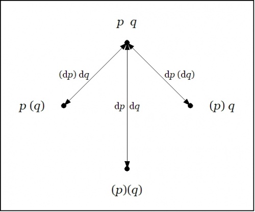
Abstracting from the augmented venn diagram that shows how the models or satisfying interpretations of \(\mathrm{D}f~\!\) distribute over the extended universe of discourse \(\mathrm{E}X = P \times Q \times \mathrm{d}P \times \mathrm{d}Q,\!\) the difference map \(\mathrm{D}f~\!\) can be represented in the form of a digraph or directed graph, one whose points are labeled with the elements of \(X = P \times Q\!\) and whose arrows are labeled with the elements of \(\mathrm{d}X = \mathrm{d}P \times \mathrm{d}Q,\!\) as shown in the following Figure.
Any proposition worth its salt can be analyzed from many different points of view, any one of which has the potential to reveal an unsuspected aspect of the proposition's meaning. We will encounter more and more of these alternative readings as we go.
The enlargement or shift operator \(\mathrm{E}\!\) exhibits a wealth of interesting and useful properties in its own right, so it pays to examine a few of the more salient features that play out on the surface of our initial example, \(f(p, q) = pq.\!\)
A suitably generic definition of the extended universe of discourse is afforded by the following set-up:
|
\(\begin{array}{lccl} \text{Let} & X & = & X_1 \times \ldots \times X_k. \\[6pt] \text{Let} & \mathrm{d}X & = & \mathrm{d}X_1 \times \ldots \times \mathrm{d}X_k. \\[6pt] \text{Then} & \mathrm{E}X & = & X \times \mathrm{d}X \\[6pt] & & = & X_1 \times \ldots \times X_k ~\times~ \mathrm{d}X_1 \times \ldots \times \mathrm{d}X_k \end{array}\!\) |
For a proposition of the form \(f : X_1 \times \ldots \times X_k \to \mathbb{B},\!\) the (first order) enlargement of \(f\!\) is the proposition \(\mathrm{E}f : \mathrm{E}X \to \mathbb{B}\!\) that is defined by the following equation:
|
\(\begin{array}{l} \mathrm{E}f(x_1, \ldots, x_k, \mathrm{d}x_1, \ldots, \mathrm{d}x_k) \\[6pt] = \quad f(x_1 + \mathrm{d}x_1, \ldots, x_k + \mathrm{d}x_k) \\[6pt] = \quad f( \texttt{(} x_1, \mathrm{d}x_1 \texttt{)}, \ldots, \texttt{(} x_k, \mathrm{d}x_k \texttt{)} ) \end{array}\!\) |
The differential variables \(\mathrm{d}x_j\!\) are boolean variables of the same basic type as the ordinary variables \(x_j.\!\) Although it is conventional to distinguish the (first order) differential variables with the operative prefix “\(\mathrm{d}\!\)” this way of notating differential variables is entirely optional. It is their existence in particular relations to the initial variables, not their names, that defines them as differential variables.
In the example of logical conjunction, \(f(p, q) = pq,\!\) the enlargement \(\mathrm{E}f\!\) is formulated as follows:
|
\(\begin{array}{l} \mathrm{E}f(p, q, \mathrm{d}p, \mathrm{d}q) \\[6pt] = \quad (p + \mathrm{d}p)(q + \mathrm{d}q) \\[6pt] = \quad \texttt{(} p, \mathrm{d}p \texttt{)(} q, \mathrm{d}q \texttt{)} \end{array}\!\) |
Given that this expression uses nothing more than the boolean ring operations of addition and multiplication, it is permissible to “multiply things out” in the usual manner to arrive at the following result:
|
\(\begin{matrix} \mathrm{E}f(p, q, \mathrm{d}p, \mathrm{d}q) & = & p~q & + & p~\mathrm{d}q & + & q~\mathrm{d}p & + & \mathrm{d}p~\mathrm{d}q \end{matrix}\!\) |
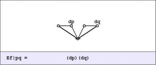
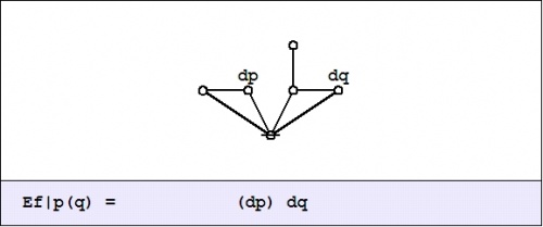
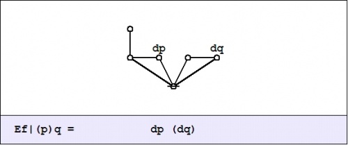
To understand what the enlarged or shifted proposition means in logical terms, it serves to go back and analyze the above expression for \(\mathrm{E}f\!\) in the same way that we did for \(\mathrm{D}f.\!\) Toward that end, the value of \(\mathrm{E}f_x\!\) at each \(x \in X\!\) may be computed in graphical fashion as shown below:

|
|
|
|

|
Given the data that develops in this form of analysis, the disjoined ingredients can now be folded back into a boolean expansion or a disjunctive normal form (DNF) that is equivalent to the enlarged proposition \(\mathrm{E}f.\!\)
|
\(\begin{matrix} \mathrm{E}f & = & pq \cdot \mathrm{E}f_{pq} & + & p(q) \cdot \mathrm{E}f_{p(q)} & + & (p)q \cdot \mathrm{E}f_{(p)q} & + & (p)(q) \cdot \mathrm{E}f_{(p)(q)} \end{matrix}\!\) |
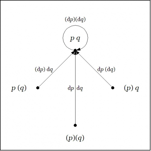
Here is a summary of the result, illustrated by means of a digraph picture, where the “no change” element \((\mathrm{d}p)(\mathrm{d}q)\!\) is drawn as a loop at the point \(p~q.\!\)
We may understand the enlarged proposition \(\mathrm{E}f\!\) as telling us all the different ways to reach a model of the proposition \(f\!\) from each point of the universe \(X.\!\)
Operational Representation
If you think that I linger in the realm of logical difference calculus out of sheer vacillation about getting down to the differential proper, it is probably out of a prior expectation that you derive from the art or the long-engrained practice of real analysis. But the fact is that ordinary calculus only rushes on to the sundry orders of approximation because the strain of comprehending the full import of \(\mathrm{E}\!\) and \(\mathrm{D}\!\) at once overwhelms its discrete and finite powers to grasp them. But here, in the fully serene idylls of zeroth order logic, we find ourselves fit with the compass of a wit that is all we'd ever need to explore their effects with care.
So let us do just that.
I will first rationalize the novel grouping of propositional forms in the last set of Tables, as that will extend a gentle invitation to the mathematical subject of group theory, and demonstrate its relevance to differential logic in a strikingly apt and useful way. The data for that account is contained in Table A3.
| \(f\!\) |
\(\mathrm{T}_{11} f\!\) \(\mathrm{E}f|_{\mathrm{d}p~\mathrm{d}q}\!\) |
\(\mathrm{T}_{10} f\!\) \(\mathrm{E}f|_{\mathrm{d}p(\mathrm{d}q)}\!\) |
\(\mathrm{T}_{01} f\!\) \(\mathrm{E}f|_{(\mathrm{d}p)\mathrm{d}q}\!\) |
\(\mathrm{T}_{00} f\!\) \(\mathrm{E}f|_{(\mathrm{d}p)(\mathrm{d}q)}\!\) | |
| \(f_0\!\) | \((~)\!\) | \((~)\!\) | \((~)\!\) | \((~)\!\) | \((~)\!\) |
|
\(\begin{matrix} f_1 \\[4pt] f_2 \\[4pt] f_4 \\[4pt] f_8 \end{matrix}\!\) |
\(\begin{matrix} (p)(q) \\[4pt] (p)~q~ \\[4pt] ~p~(q) \\[4pt] ~p~~q~ \end{matrix}\!\) |
\(\begin{matrix} ~p~~q~ \\[4pt] ~p~(q) \\[4pt] (p)~q~ \\[4pt] (p)(q) \end{matrix}\!\) |
\(\begin{matrix} ~p~(q) \\[4pt] ~p~~q~ \\[4pt] (p)(q) \\[4pt] (p)~q~ \end{matrix}\!\) |
\(\begin{matrix} (p)~q~ \\[4pt] (p)(q) \\[4pt] ~p~~q~ \\[4pt] ~p~(q) \end{matrix}\!\) |
\(\begin{matrix} (p)(q) \\[4pt] (p)~q~ \\[4pt] ~p~(q) \\[4pt] ~p~~q~ \end{matrix}\!\) |
|
\(\begin{matrix} f_3 \\[4pt] f_{12} \end{matrix}\!\) |
\(\begin{matrix} (p) \\[4pt] ~p~ \end{matrix}\!\) |
\(\begin{matrix} ~p~ \\[4pt] (p) \end{matrix}\!\) |
\(\begin{matrix} ~p~ \\[4pt] (p) \end{matrix}\!\) |
\(\begin{matrix} (p) \\[4pt] ~p~ \end{matrix}\!\) |
\(\begin{matrix} (p) \\[4pt] ~p~ \end{matrix}\!\) |
|
\(\begin{matrix} f_6 \\[4pt] f_9 \end{matrix}\!\) |
\(\begin{matrix} ~(p,~q)~ \\[4pt] ((p,~q)) \end{matrix}\!\) |
\(\begin{matrix} ~(p,~q)~ \\[4pt] ((p,~q)) \end{matrix}\!\) |
\(\begin{matrix} ((p,~q)) \\[4pt] ~(p,~q)~ \end{matrix}\!\) |
\(\begin{matrix} ((p,~q)) \\[4pt] ~(p,~q)~ \end{matrix}\!\) |
\(\begin{matrix} ~(p,~q)~ \\[4pt] ((p,~q)) \end{matrix}\!\) |
|
\(\begin{matrix} f_5 \\[4pt] f_{10} \end{matrix}\!\) |
\(\begin{matrix} (q) \\[4pt] ~q~ \end{matrix}\!\) |
\(\begin{matrix} ~q~ \\[4pt] (q) \end{matrix}\!\) |
\(\begin{matrix} (q) \\[4pt] ~q~ \end{matrix}\!\) |
\(\begin{matrix} ~q~ \\[4pt] (q) \end{matrix}\!\) |
\(\begin{matrix} (q) \\[4pt] ~q~ \end{matrix}\!\) |
|
\(\begin{matrix} f_7 \\[4pt] f_{11} \\[4pt] f_{13} \\[4pt] f_{14} \end{matrix}\!\) |
\(\begin{matrix} (~p~~q~) \\[4pt] (~p~(q)) \\[4pt] ((p)~q~) \\[4pt] ((p)(q)) \end{matrix}\!\) |
\(\begin{matrix} ((p)(q)) \\[4pt] ((p)~q~) \\[4pt] (~p~(q)) \\[4pt] (~p~~q~) \end{matrix}\!\) |
\(\begin{matrix} ((p)~q~) \\[4pt] ((p)(q)) \\[4pt] (~p~~q~) \\[4pt] (~p~(q)) \end{matrix}\!\) |
\(\begin{matrix} (~p~(q)) \\[4pt] (~p~~q~) \\[4pt] ((p)(q)) \\[4pt] ((p)~q~) \end{matrix}\!\) |
\(\begin{matrix} (~p~~q~) \\[4pt] (~p~(q)) \\[4pt] ((p)~q~) \\[4pt] ((p)(q)) \end{matrix}\!\) |
| \(f_{15}\!\) | \(((~))\!\) | \(((~))\!\) | \(((~))\!\) | \(((~))\!\) | \(((~))\!\) |
| \(\text{Fixed Point Total}\!\) | \(4\!\) | \(4\!\) | \(4\!\) | \(16\!\) | |
The shift operator \(\mathrm{E}\!\) can be understood as enacting a substitution operation on the propositional form \(f(p, q)\!\) that is given as its argument. In our present focus on propositional forms that involve two variables, we have the following type specifications and definitions:
|
\(\begin{array}{lcl} \mathrm{E} ~:~ (X \to \mathbb{B}) & \to & (\mathrm{E}X \to \mathbb{B}) \\[6pt] \mathrm{E} ~:~ f(p, q) & \mapsto & \mathrm{E}f(p, q, \mathrm{d}p, \mathrm{d}q) \\[6pt] \mathrm{E}f(p, q, \mathrm{d}p, \mathrm{d}q) & = & f(p + \mathrm{d}p, q + \mathrm{d}q) \\[6pt] & = & f( \texttt{(} p, \mathrm{d}p \texttt{)}, \texttt{(} q, \mathrm{d}q \texttt{)} ) \end{array}\!\) |
Evaluating \(\mathrm{E}f\!\) at particular values of \(\mathrm{d}p\!\) and \(\mathrm{d}q,\!\) for example, \(\mathrm{d}p = i\!\) and \(\mathrm{d}q = j,\!\) where \(i\!\) and \(j\!\) are values in \(\mathbb{B},\!\) produces the following result:
|
\(\begin{array}{lclcl} \mathrm{E}_{ij} & : & (X \to \mathbb{B}) & \to & (X \to \mathbb{B}) \\[6pt] \mathrm{E}_{ij} & : & f & \mapsto & \mathrm{E}_{ij}f \\[6pt] \mathrm{E}_{ij}f & = & \mathrm{E}f|_{\mathrm{d}p = i, \mathrm{d}q = j} & = & f(p + i, q + j) \\[6pt] & & & = & f( \texttt{(} p, i \texttt{)}, \texttt{(} q, j \texttt{)} ) \end{array}\!\) |
The notation is a little awkward, but the data of Table A3 should make the sense clear. The important thing to observe is that \(\mathrm{E}_{ij}\!\) has the effect of transforming each proposition \(f : X \to \mathbb{B}\!\) into a proposition \(f^\prime : X \to \mathbb{B}.\!\) As it happens, the action of each \(\mathrm{E}_{ij}\!\) is one-to-one and onto, so the gang of four operators \(\{ \mathrm{E}_{ij} : i, j \in \mathbb{B} \}\!\) is an example of what is called a transformation group on the set of sixteen propositions. Bowing to a longstanding local and linear tradition, I will therefore redub the four elements of this group as \(\mathrm{T}_{00}, \mathrm{T}_{01}, \mathrm{T}_{10}, \mathrm{T}_{11},\!\) to bear in mind their transformative character, or nature, as the case may be. Abstractly viewed, this group of order four has the following operation table:
|
\(\cdot\!\) |
\(\mathrm{T}_{00}\!\) |
\(\mathrm{T}_{01}\!\) |
\(\mathrm{T}_{10}\!\) |
\(\mathrm{T}_{11}\!\) |
| \(\mathrm{T}_{00}\!\) | \(\mathrm{T}_{00}\!\) | \(\mathrm{T}_{01}\!\) | \(\mathrm{T}_{10}\!\) | \(\mathrm{T}_{11}\!\) |
| \(\mathrm{T}_{01}\!\) | \(\mathrm{T}_{01}\!\) | \(\mathrm{T}_{00}\!\) | \(\mathrm{T}_{11}\!\) | \(\mathrm{T}_{10}\!\) |
| \(\mathrm{T}_{10}\!\) | \(\mathrm{T}_{10}\!\) | \(\mathrm{T}_{11}\!\) | \(\mathrm{T}_{00}\!\) | \(\mathrm{T}_{01}\!\) |
| \(\mathrm{T}_{11}\!\) | \(\mathrm{T}_{11}\!\) | \(\mathrm{T}_{10}\!\) | \(\mathrm{T}_{01}\!\) | \(\mathrm{T}_{00}\!\) |
It happens that there are just two possible groups of 4 elements. One is the cyclic group \(Z_4\!\) (from German Zyklus), which this is not. The other is the Klein four-group \(V_4\!\) (from German Vier), which this is.
More concretely viewed, the group as a whole pushes the set of sixteen propositions around in such a way that they fall into seven natural classes, called orbits. One says that the orbits are preserved by the action of the group. There is an Orbit Lemma of immense utility to “those who count” which, depending on your upbringing, you may associate with the names of Burnside, Cauchy, Frobenius, or some subset or superset of these three, vouching that the number of orbits is equal to the mean number of fixed points, in other words, the total number of points (in our case, propositions) that are left unmoved by the separate operations, divided by the order of the group.
Propositional Forms on Two Variables
To broaden our experience with simple examples, let us examine the sixteen functions of concrete type \(P \times Q \to \mathbb{B}\!\) and abstract type \(\mathbb{B} \times \mathbb{B} \to \mathbb{B}.\!\) A few Tables are set here that detail the actions of \(\mathrm{E}\!\) and \(\mathrm{D}\!\) on each of these functions, allowing us to view the results in several different ways.
Tables A1 and A2 show two ways of arranging the 16 boolean functions on two variables, giving equivalent expressions for each function in several different systems of notation.
|
\(\mathcal{L}_1\!\) \(\text{Decimal}\!\) |
\(\mathcal{L}_2\!\) \(\text{Binary}\!\) |
\(\mathcal{L}_3\!\) \(\text{Vector}\!\) |
\(\mathcal{L}_4\!\) \(\text{Cactus}\!\) |
\(\mathcal{L}_5\!\) \(\text{English}\!\) |
\(\mathcal{L}_6~\!\) \(\text{Ordinary}\!\) |
| \(p\colon\!\) | \(1~1~0~0\!\) | ||||
| \(q\colon\!\) | \(1~0~1~0\!\) | ||||
|
\(\begin{matrix} f_0 \\[4pt] f_1 \\[4pt] f_2 \\[4pt] f_3 \\[4pt] f_4 \\[4pt] f_5 \\[4pt] f_6 \\[4pt] f_7 \end{matrix}\!\) |
\(\begin{matrix} f_{0000} \\[4pt] f_{0001} \\[4pt] f_{0010} \\[4pt] f_{0011} \\[4pt] f_{0100} \\[4pt] f_{0101} \\[4pt] f_{0110} \\[4pt] f_{0111} \end{matrix}\!\) |
\(\begin{matrix} 0~0~0~0 \\[4pt] 0~0~0~1 \\[4pt] 0~0~1~0 \\[4pt] 0~0~1~1 \\[4pt] 0~1~0~0 \\[4pt] 0~1~0~1 \\[4pt] 0~1~1~0 \\[4pt] 0~1~1~1 \end{matrix}\!\) |
\(\begin{matrix} (~) \\[4pt] (p)(q) \\[4pt] (p)~q~ \\[4pt] (p)~ ~ \\[4pt] ~p~(q) \\[4pt] ~ ~(q) \\[4pt] (p,~q) \\[4pt] (p~~q) \end{matrix}\!\) |
\(\begin{matrix} \text{false} \\[4pt] \text{neither}~ p ~\text{nor}~ q \\[4pt] q ~\text{without}~ p \\[4pt] \text{not}~ p \\[4pt] p ~\text{without}~ q \\[4pt] \text{not}~ q \\[4pt] p ~\text{not equal to}~ q \\[4pt] \text{not both}~ p ~\text{and}~ q \end{matrix}\!\) |
\(\begin{matrix} 0 \\[4pt] \lnot p \land \lnot q \\[4pt] \lnot p \land q \\[4pt] \lnot p \\[4pt] p \land \lnot q \\[4pt] \lnot q \\[4pt] p \ne q \\[4pt] \lnot p \lor \lnot q \end{matrix}\!\) |
|
\(\begin{matrix} f_8 \\[4pt] f_9 \\[4pt] f_{10} \\[4pt] f_{11} \\[4pt] f_{12} \\[4pt] f_{13} \\[4pt] f_{14} \\[4pt] f_{15} \end{matrix}\!\) |
\(\begin{matrix} f_{1000} \\[4pt] f_{1001} \\[4pt] f_{1010} \\[4pt] f_{1011} \\[4pt] f_{1100} \\[4pt] f_{1101} \\[4pt] f_{1110} \\[4pt] f_{1111} \end{matrix}\!\) |
\(\begin{matrix} 1~0~0~0 \\[4pt] 1~0~0~1 \\[4pt] 1~0~1~0 \\[4pt] 1~0~1~1 \\[4pt] 1~1~0~0 \\[4pt] 1~1~0~1 \\[4pt] 1~1~1~0 \\[4pt] 1~1~1~1 \end{matrix}\!\) |
\(\begin{matrix} ~~p~~q~~ \\[4pt] ((p,~q)) \\[4pt] ~ ~ ~q~~ \\[4pt] ~(p~(q)) \\[4pt] ~~p~ ~ ~ \\[4pt] ((p)~q)~ \\[4pt] ((p)(q)) \\[4pt] ((~)) \end{matrix}\!\) |
\(\begin{matrix} p ~\text{and}~ q \\[4pt] p ~\text{equal to}~ q \\[4pt] q \\[4pt] \text{not}~ p ~\text{without}~ q \\[4pt] p \\[4pt] \text{not}~ q ~\text{without}~ p \\[4pt] p ~\text{or}~ q \\[4pt] \text{true} \end{matrix}\!\) |
\(\begin{matrix} p \land q \\[4pt] p = q \\[4pt] q \\[4pt] p \Rightarrow q \\[4pt] p \\[4pt] p \Leftarrow q \\[4pt] p \lor q \\[4pt] 1 \end{matrix}\!\) |
|
\(\mathcal{L}_1\!\) \(\text{Decimal}\!\) |
\(\mathcal{L}_2\!\) \(\text{Binary}\!\) |
\(\mathcal{L}_3\!\) \(\text{Vector}\!\) |
\(\mathcal{L}_4\!\) \(\text{Cactus}\!\) |
\(\mathcal{L}_5\!\) \(\text{English}\!\) |
\(\mathcal{L}_6~\!\) \(\text{Ordinary}\!\) |
| \(p\colon\!\) | \(1~1~0~0\!\) | ||||
| \(q\colon\!\) | \(1~0~1~0\!\) | ||||
| \(f_0\!\) | \(f_{0000}\!\) | \(0~0~0~0\!\) | \((~)\!\) | \(\text{false}\!\) | \(0\!\) |
|
\(\begin{matrix} f_1 \\[4pt] f_2 \\[4pt] f_4 \\[4pt] f_8 \end{matrix}\!\) |
\(\begin{matrix} f_{0001} \\[4pt] f_{0010} \\[4pt] f_{0100} \\[4pt] f_{1000} \end{matrix}\!\) |
\(\begin{matrix} 0~0~0~1 \\[4pt] 0~0~1~0 \\[4pt] 0~1~0~0 \\[4pt] 1~0~0~0 \end{matrix}\!\) |
\(\begin{matrix} (p)(q) \\[4pt] (p)~q~ \\[4pt] ~p~(q) \\[4pt] ~p~~q~ \end{matrix}\!\) |
\(\begin{matrix} \text{neither}~ p ~\text{nor}~ q \\[4pt] q ~\text{without}~ p \\[4pt] p ~\text{without}~ q \\[4pt] p ~\text{and}~ q \end{matrix}\!\) |
\(\begin{matrix} \lnot p \land \lnot q \\[4pt] \lnot p \land q \\[4pt] p \land \lnot q \\[4pt] p \land q \end{matrix}\!\) |
|
\(\begin{matrix} f_3 \\[4pt] f_{12} \end{matrix}\!\) |
\(\begin{matrix} f_{0011} \\[4pt] f_{1100} \end{matrix}\!\) |
\(\begin{matrix} 0~0~1~1 \\[4pt] 1~1~0~0 \end{matrix}\!\) |
\(\begin{matrix} (p) \\[4pt] ~p~ \end{matrix}\!\) |
\(\begin{matrix} \text{not}~ p \\[4pt] p \end{matrix}\!\) |
\(\begin{matrix} \lnot p \\[4pt] p \end{matrix}\!\) |
|
\(\begin{matrix} f_6 \\[4pt] f_9 \end{matrix}\!\) |
\(\begin{matrix} f_{0110} \\[4pt] f_{1001} \end{matrix}\!\) |
\(\begin{matrix} 0~1~1~0 \\[4pt] 1~0~0~1 \end{matrix}\!\) |
\(\begin{matrix} ~(p,~q)~ \\[4pt] ((p,~q)) \end{matrix}\!\) |
\(\begin{matrix} p ~\text{not equal to}~ q \\[4pt] p ~\text{equal to}~ q \end{matrix}\!\) |
\(\begin{matrix} p \ne q \\[4pt] p = q \end{matrix}\!\) |
|
\(\begin{matrix} f_5 \\[4pt] f_{10} \end{matrix}\!\) |
\(\begin{matrix} f_{0101} \\[4pt] f_{1010} \end{matrix}\!\) |
\(\begin{matrix} 0~1~0~1 \\[4pt] 1~0~1~0 \end{matrix}\!\) |
\(\begin{matrix} (q) \\[4pt] ~q~ \end{matrix}\!\) |
\(\begin{matrix} \text{not}~ q \\[4pt] q \end{matrix}\!\) |
\(\begin{matrix} \lnot q \\[4pt] q \end{matrix}\!\) |
|
\(\begin{matrix} f_7 \\[4pt] f_{11} \\[4pt] f_{13} \\[4pt] f_{14} \end{matrix}\!\) |
\(\begin{matrix} f_{0111} \\[4pt] f_{1011} \\[4pt] f_{1101} \\[4pt] f_{1110} \end{matrix}\!\) |
\(\begin{matrix} 0~1~1~1 \\[4pt] 1~0~1~1 \\[4pt] 1~1~0~1 \\[4pt] 1~1~1~0 \end{matrix}\!\) |
\(\begin{matrix} ~(p~~q)~ \\[4pt] ~(p~(q)) \\[4pt] ((p)~q)~ \\[4pt] ((p)(q)) \end{matrix}\!\) |
\(\begin{matrix} \text{not both}~ p ~\text{and}~ q \\[4pt] \text{not}~ p ~\text{without}~ q \\[4pt] \text{not}~ q ~\text{without}~ p \\[4pt] p ~\text{or}~ q \end{matrix}\!\) |
\(\begin{matrix} \lnot p \lor \lnot q \\[4pt] p \Rightarrow q \\[4pt] p \Leftarrow q \\[4pt] p \lor q \end{matrix}\!\) |
| \(f_{15}\!\) | \(f_{1111}\!\) | \(1~1~1~1\!\) | \(((~))\!\) | \(\text{true}\!\) | \(1\!\) |
Transforms Expanded over Differential Features
The next four Tables expand the expressions of \(\mathrm{E}f\!\) and \(\mathrm{D}f~\!\) in two different ways, for each of the sixteen functions. Notice that the functions are given in a different order, partitioned into seven natural classes by a group action.
| \(f\!\) |
\(\mathrm{T}_{11} f\!\) \(\mathrm{E}f|_{\mathrm{d}p~\mathrm{d}q}\!\) |
\(\mathrm{T}_{10} f\!\) \(\mathrm{E}f|_{\mathrm{d}p(\mathrm{d}q)}\!\) |
\(\mathrm{T}_{01} f\!\) \(\mathrm{E}f|_{(\mathrm{d}p)\mathrm{d}q}\!\) |
\(\mathrm{T}_{00} f\!\) \(\mathrm{E}f|_{(\mathrm{d}p)(\mathrm{d}q)}\!\) | |
| \(f_0\!\) | \((~)\!\) | \((~)\!\) | \((~)\!\) | \((~)\!\) | \((~)\!\) |
|
\(\begin{matrix} f_1 \\[4pt] f_2 \\[4pt] f_4 \\[4pt] f_8 \end{matrix}\!\) |
\(\begin{matrix} (p)(q) \\[4pt] (p)~q~ \\[4pt] ~p~(q) \\[4pt] ~p~~q~ \end{matrix}\!\) |
\(\begin{matrix} ~p~~q~ \\[4pt] ~p~(q) \\[4pt] (p)~q~ \\[4pt] (p)(q) \end{matrix}\!\) |
\(\begin{matrix} ~p~(q) \\[4pt] ~p~~q~ \\[4pt] (p)(q) \\[4pt] (p)~q~ \end{matrix}\!\) |
\(\begin{matrix} (p)~q~ \\[4pt] (p)(q) \\[4pt] ~p~~q~ \\[4pt] ~p~(q) \end{matrix}\!\) |
\(\begin{matrix} (p)(q) \\[4pt] (p)~q~ \\[4pt] ~p~(q) \\[4pt] ~p~~q~ \end{matrix}\!\) |
|
\(\begin{matrix} f_3 \\[4pt] f_{12} \end{matrix}\!\) |
\(\begin{matrix} (p) \\[4pt] ~p~ \end{matrix}\!\) |
\(\begin{matrix} ~p~ \\[4pt] (p) \end{matrix}\!\) |
\(\begin{matrix} ~p~ \\[4pt] (p) \end{matrix}\!\) |
\(\begin{matrix} (p) \\[4pt] ~p~ \end{matrix}\!\) |
\(\begin{matrix} (p) \\[4pt] ~p~ \end{matrix}\!\) |
|
\(\begin{matrix} f_6 \\[4pt] f_9 \end{matrix}\!\) |
\(\begin{matrix} ~(p,~q)~ \\[4pt] ((p,~q)) \end{matrix}\!\) |
\(\begin{matrix} ~(p,~q)~ \\[4pt] ((p,~q)) \end{matrix}\!\) |
\(\begin{matrix} ((p,~q)) \\[4pt] ~(p,~q)~ \end{matrix}\!\) |
\(\begin{matrix} ((p,~q)) \\[4pt] ~(p,~q)~ \end{matrix}\!\) |
\(\begin{matrix} ~(p,~q)~ \\[4pt] ((p,~q)) \end{matrix}\!\) |
|
\(\begin{matrix} f_5 \\[4pt] f_{10} \end{matrix}\!\) |
\(\begin{matrix} (q) \\[4pt] ~q~ \end{matrix}\!\) |
\(\begin{matrix} ~q~ \\[4pt] (q) \end{matrix}\!\) |
\(\begin{matrix} (q) \\[4pt] ~q~ \end{matrix}\!\) |
\(\begin{matrix} ~q~ \\[4pt] (q) \end{matrix}\!\) |
\(\begin{matrix} (q) \\[4pt] ~q~ \end{matrix}\!\) |
|
\(\begin{matrix} f_7 \\[4pt] f_{11} \\[4pt] f_{13} \\[4pt] f_{14} \end{matrix}\!\) |
\(\begin{matrix} (~p~~q~) \\[4pt] (~p~(q)) \\[4pt] ((p)~q~) \\[4pt] ((p)(q)) \end{matrix}\!\) |
\(\begin{matrix} ((p)(q)) \\[4pt] ((p)~q~) \\[4pt] (~p~(q)) \\[4pt] (~p~~q~) \end{matrix}\!\) |
\(\begin{matrix} ((p)~q~) \\[4pt] ((p)(q)) \\[4pt] (~p~~q~) \\[4pt] (~p~(q)) \end{matrix}\!\) |
\(\begin{matrix} (~p~(q)) \\[4pt] (~p~~q~) \\[4pt] ((p)(q)) \\[4pt] ((p)~q~) \end{matrix}\!\) |
\(\begin{matrix} (~p~~q~) \\[4pt] (~p~(q)) \\[4pt] ((p)~q~) \\[4pt] ((p)(q)) \end{matrix}\!\) |
| \(f_{15}\!\) | \(((~))\!\) | \(((~))\!\) | \(((~))\!\) | \(((~))\!\) | \(((~))\!\) |
| \(\text{Fixed Point Total}\!\) | \(4\!\) | \(4\!\) | \(4\!\) | \(16\!\) | |
| \(f\!\) |
\(\mathrm{D}f|_{\mathrm{d}p~\mathrm{d}q}\!\) |
\(\mathrm{D}f|_{\mathrm{d}p(\mathrm{d}q)}\!\) |
\(\mathrm{D}f|_{(\mathrm{d}p)\mathrm{d}q}\!\) |
\(\mathrm{D}f|_{(\mathrm{d}p)(\mathrm{d}q)}\!\) | |
| \(f_0\!\) | \((~)\!\) | \((~)\!\) | \((~)\!\) | \((~)\!\) | \((~)\!\) |
|
\(\begin{matrix} f_1 \\[4pt] f_2 \\[4pt] f_4 \\[4pt] f_8 \end{matrix}\!\) |
\(\begin{matrix} (p)(q) \\[4pt] (p)~q~ \\[4pt] ~p~(q) \\[4pt] ~p~~q~ \end{matrix}\!\) |
\(\begin{matrix} ((p,~q)) \\[4pt] ~(p,~q)~ \\[4pt] ~(p,~q)~ \\[4pt] ((p,~q)) \end{matrix}\!\) |
\(\begin{matrix} (q) \\[4pt] ~q~ \\[4pt] (q) \\[4pt] ~q~ \end{matrix}\!\) |
\(\begin{matrix} (p) \\[4pt] (p) \\[4pt] ~p~ \\[4pt] ~p~ \end{matrix}\!\) |
\(\begin{matrix} (~) \\[4pt] (~) \\[4pt] (~) \\[4pt] (~) \end{matrix}\!\) |
|
\(\begin{matrix} f_3 \\[4pt] f_{12} \end{matrix}\!\) |
\(\begin{matrix} (p) \\[4pt] ~p~ \end{matrix}\!\) |
\(\begin{matrix} ((~)) \\[4pt] ((~)) \end{matrix}~\!\) |
\(\begin{matrix} ((~)) \\[4pt] ((~)) \end{matrix}~\!\) |
\(\begin{matrix} (~) \\[4pt] (~) \end{matrix}\!\) |
\(\begin{matrix} (~) \\[4pt] (~) \end{matrix}\!\) |
|
\(\begin{matrix} f_6 \\[4pt] f_9 \end{matrix}\!\) |
\(\begin{matrix} ~(p,~q)~ \\[4pt] ((p,~q)) \end{matrix}\!\) |
\(\begin{matrix} (~) \\[4pt] (~) \end{matrix}\!\) |
\(\begin{matrix} ((~)) \\[4pt] ((~)) \end{matrix}~\!\) |
\(\begin{matrix} ((~)) \\[4pt] ((~)) \end{matrix}~\!\) |
\(\begin{matrix} (~) \\[4pt] (~) \end{matrix}\!\) |
|
\(\begin{matrix} f_5 \\[4pt] f_{10} \end{matrix}\!\) |
\(\begin{matrix} (q) \\[4pt] ~q~ \end{matrix}\!\) |
\(\begin{matrix} ((~)) \\[4pt] ((~)) \end{matrix}~\!\) |
\(\begin{matrix} (~) \\[4pt] (~) \end{matrix}\!\) |
\(\begin{matrix} ((~)) \\[4pt] ((~)) \end{matrix}~\!\) |
\(\begin{matrix} (~) \\[4pt] (~) \end{matrix}\!\) |
|
\(\begin{matrix} f_7 \\[4pt] f_{11} \\[4pt] f_{13} \\[4pt] f_{14} \end{matrix}\!\) |
\(\begin{matrix} ~(p~~q)~ \\[4pt] ~(p~(q)) \\[4pt] ((p)~q)~ \\[4pt] ((p)(q)) \end{matrix}\!\) |
\(\begin{matrix} ((p,~q)) \\[4pt] ~(p,~q)~ \\[4pt] ~(p,~q)~ \\[4pt] ((p,~q)) \end{matrix}\!\) |
\(\begin{matrix} ~q~ \\[4pt] (q) \\[4pt] ~q~ \\[4pt] (q) \end{matrix}\!\) |
\(\begin{matrix} ~p~ \\[4pt] ~p~ \\[4pt] (p) \\[4pt] (p) \end{matrix}\!\) |
\(\begin{matrix} (~) \\[4pt] (~) \\[4pt] (~) \\[4pt] (~) \end{matrix}\!\) |
| \(f_{15}\!\) | \(((~))\!\) | \((~)\!\) | \((~)\!\) | \((~)\!\) | \((~)\!\) |
Transforms Expanded over Ordinary Features
| \(f\!\) | \(\mathrm{E}f|_{pq}\!\) | \(\mathrm{E}f|_{p(q)}\!\) | \(\mathrm{E}f|_{(p)q}\!\) | \(\mathrm{E}f|_{(p)(q)}\!\) | |
| \(f_0\!\) | \((~)\!\) | \((~)\!\) | \((~)\!\) | \((~)\!\) | \((~)\!\) |
|
\(\begin{matrix} f_1 \\[4pt] f_2 \\[4pt] f_4 \\[4pt] f_8 \end{matrix}\!\) |
\(\begin{matrix} (p)(q) \\[4pt] (p)~q~ \\[4pt] ~p~(q) \\[4pt] ~p~~q~ \end{matrix}\!\) |
\(\begin{matrix} ~\mathrm{d}p~~\mathrm{d}q~ \\[4pt] ~\mathrm{d}p~(\mathrm{d}q) \\[4pt] (\mathrm{d}p)~\mathrm{d}q~ \\[4pt] (\mathrm{d}p)(\mathrm{d}q) \end{matrix}\!\) |
\(\begin{matrix} ~\mathrm{d}p~(\mathrm{d}q) \\[4pt] ~\mathrm{d}p~~\mathrm{d}q~ \\[4pt] (\mathrm{d}p)(\mathrm{d}q) \\[4pt] (\mathrm{d}p)~\mathrm{d}q~ \end{matrix}\!\) |
\(\begin{matrix} (\mathrm{d}p)~\mathrm{d}q~ \\[4pt] (\mathrm{d}p)(\mathrm{d}q) \\[4pt] ~\mathrm{d}p~~\mathrm{d}q~ \\[4pt] ~\mathrm{d}p~(\mathrm{d}q) \end{matrix}\!\) |
\(\begin{matrix} (\mathrm{d}p)(\mathrm{d}q) \\[4pt] (\mathrm{d}p)~\mathrm{d}q~ \\[4pt] ~\mathrm{d}p~(\mathrm{d}q) \\[4pt] ~\mathrm{d}p~~\mathrm{d}q~ \end{matrix}\!\) |
|
\(\begin{matrix} f_3 \\[4pt] f_{12} \end{matrix}\!\) |
\(\begin{matrix} (p) \\[4pt] ~p~ \end{matrix}\!\) |
\(\begin{matrix} ~\mathrm{d}p~ \\[4pt] (\mathrm{d}p) \end{matrix}\!\) |
\(\begin{matrix} ~\mathrm{d}p~ \\[4pt] (\mathrm{d}p) \end{matrix}\!\) |
\(\begin{matrix} (\mathrm{d}p) \\[4pt] ~\mathrm{d}p~ \end{matrix}~\!\) |
\(\begin{matrix} (\mathrm{d}p) \\[4pt] ~\mathrm{d}p~ \end{matrix}~\!\) |
|
\(\begin{matrix} f_6 \\[4pt] f_9 \end{matrix}\!\) |
\(\begin{matrix} ~(p,~q)~ \\[4pt] ((p,~q)) \end{matrix}\!\) |
\(\begin{matrix} ~(\mathrm{d}p,~\mathrm{d}q)~ \\[4pt] ((\mathrm{d}p,~\mathrm{d}q)) \end{matrix}\!\) |
\(\begin{matrix} ((\mathrm{d}p,~\mathrm{d}q)) \\[4pt] ~(\mathrm{d}p,~\mathrm{d}q)~ \end{matrix}\!\) |
\(\begin{matrix} ((\mathrm{d}p,~\mathrm{d}q)) \\[4pt] ~(\mathrm{d}p,~\mathrm{d}q)~ \end{matrix}\!\) |
\(\begin{matrix} ~(\mathrm{d}p,~\mathrm{d}q)~ \\[4pt] ((\mathrm{d}p,~\mathrm{d}q)) \end{matrix}\!\) |
|
\(\begin{matrix} f_5 \\[4pt] f_{10} \end{matrix}\!\) |
\(\begin{matrix} (q) \\[4pt] ~q~ \end{matrix}\!\) |
\(\begin{matrix} ~\mathrm{d}q~ \\[4pt] (\mathrm{d}q) \end{matrix}\!\) |
\(\begin{matrix} (\mathrm{d}q) \\[4pt] ~\mathrm{d}q~ \end{matrix}\!\) |
\(\begin{matrix} ~\mathrm{d}q~ \\[4pt] (\mathrm{d}q) \end{matrix}\!\) |
\(\begin{matrix} (\mathrm{d}q) \\[4pt] ~\mathrm{d}q~ \end{matrix}\!\) |
|
\(\begin{matrix} f_7 \\[4pt] f_{11} \\[4pt] f_{13} \\[4pt] f_{14} \end{matrix}\!\) |
\(\begin{matrix} (~p~~q~) \\[4pt] (~p~(q)) \\[4pt] ((p)~q~) \\[4pt] ((p)(q)) \end{matrix}\!\) |
\(\begin{matrix} ((\mathrm{d}p)(\mathrm{d}q)) \\[4pt] ((\mathrm{d}p)~\mathrm{d}q~) \\[4pt] (~\mathrm{d}p~(\mathrm{d}q)) \\[4pt] (~\mathrm{d}p~~\mathrm{d}q~) \end{matrix}\!\) |
\(\begin{matrix} ((\mathrm{d}p)~\mathrm{d}q~) \\[4pt] ((\mathrm{d}p)(\mathrm{d}q)) \\[4pt] (~\mathrm{d}p~~\mathrm{d}q~) \\[4pt] (~\mathrm{d}p~(\mathrm{d}q)) \end{matrix}\!\) |
\(\begin{matrix} (~\mathrm{d}p~(\mathrm{d}q)) \\[4pt] (~\mathrm{d}p~~\mathrm{d}q~) \\[4pt] ((\mathrm{d}p)(\mathrm{d}q)) \\[4pt] ((\mathrm{d}p)~\mathrm{d}q~) \end{matrix}\!\) |
\(\begin{matrix} (~\mathrm{d}p~~\mathrm{d}q~) \\[4pt] (~\mathrm{d}p~(\mathrm{d}q)) \\[4pt] ((\mathrm{d}p)~\mathrm{d}q~) \\[4pt] ((\mathrm{d}p)(\mathrm{d}q)) \end{matrix}\!\) |
| \(f_{15}\!\) | \(((~))\!\) | \(((~))\!\) | \(((~))\!\) | \(((~))\!\) | \(((~))\!\) |
| \(f\!\) | \(\mathrm{D}f|_{pq}\!\) | \(\mathrm{D}f|_{p(q)}\!\) | \(\mathrm{D}f|_{(p)q}\!\) | \(\mathrm{D}f|_{(p)(q)}\!\) | |
| \(f_0\!\) | \((~)\!\) | \((~)\!\) | \((~)\!\) | \((~)\!\) | \((~)\!\) |
|
\(\begin{matrix} f_1 \\[4pt] f_2 \\[4pt] f_4 \\[4pt] f_8 \end{matrix}\!\) |
\(\begin{matrix} (p)(q) \\[4pt] (p)~q~ \\[4pt] ~p~(q) \\[4pt] ~p~~q~ \end{matrix}\!\) |
\(\begin{matrix} ~~\mathrm{d}p~~\mathrm{d}q~~ \\[4pt] ~~\mathrm{d}p~(\mathrm{d}q)~ \\[4pt] ~(\mathrm{d}p)~\mathrm{d}q~~ \\[4pt] ((\mathrm{d}p)(\mathrm{d}q)) \end{matrix}\!\) |
\(\begin{matrix} ~~\mathrm{d}p~(\mathrm{d}q)~ \\[4pt] ~~\mathrm{d}p~~\mathrm{d}q~~ \\[4pt] ((\mathrm{d}p)(\mathrm{d}q)) \\[4pt] ~(\mathrm{d}p)~\mathrm{d}q~~ \end{matrix}\!\) |
\(\begin{matrix} ~(\mathrm{d}p)~\mathrm{d}q~~ \\[4pt] ((\mathrm{d}p)(\mathrm{d}q)) \\[4pt] ~~\mathrm{d}p~~\mathrm{d}q~~ \\[4pt] ~~\mathrm{d}p~(\mathrm{d}q)~ \end{matrix}\!\) |
\(\begin{matrix} ((\mathrm{d}p)(\mathrm{d}q)) \\[4pt] ~(\mathrm{d}p)~\mathrm{d}q~~ \\[4pt] ~~\mathrm{d}p~(\mathrm{d}q)~ \\[4pt] ~~\mathrm{d}p~~\mathrm{d}q~~ \end{matrix}\!\) |
|
\(\begin{matrix} f_3 \\[4pt] f_{12} \end{matrix}\!\) |
\(\begin{matrix} (p) \\[4pt] ~p~ \end{matrix}\!\) |
\(\begin{matrix} \mathrm{d}p \\[4pt] \mathrm{d}p \end{matrix}\!\) |
\(\begin{matrix} \mathrm{d}p \\[4pt] \mathrm{d}p \end{matrix}\!\) |
\(\begin{matrix} \mathrm{d}p \\[4pt] \mathrm{d}p \end{matrix}\!\) |
\(\begin{matrix} \mathrm{d}p \\[4pt] \mathrm{d}p \end{matrix}\!\) |
|
\(\begin{matrix} f_6 \\[4pt] f_9 \end{matrix}\!\) |
\(\begin{matrix} ~(p,~q)~ \\[4pt] ((p,~q)) \end{matrix}\!\) |
\(\begin{matrix} (\mathrm{d}p,~\mathrm{d}q) \\[4pt] (\mathrm{d}p,~\mathrm{d}q) \end{matrix}\!\) |
\(\begin{matrix} (\mathrm{d}p,~\mathrm{d}q) \\[4pt] (\mathrm{d}p,~\mathrm{d}q) \end{matrix}\!\) |
\(\begin{matrix} (\mathrm{d}p,~\mathrm{d}q) \\[4pt] (\mathrm{d}p,~\mathrm{d}q) \end{matrix}\!\) |
\(\begin{matrix} (\mathrm{d}p,~\mathrm{d}q) \\[4pt] (\mathrm{d}p,~\mathrm{d}q) \end{matrix}\!\) |
|
\(\begin{matrix} f_5 \\[4pt] f_{10} \end{matrix}\!\) |
\(\begin{matrix} (q) \\[4pt] ~q~ \end{matrix}\!\) |
\(\begin{matrix} \mathrm{d}q \\[4pt] \mathrm{d}q \end{matrix}\!\) |
\(\begin{matrix} \mathrm{d}q \\[4pt] \mathrm{d}q \end{matrix}\!\) |
\(\begin{matrix} \mathrm{d}q \\[4pt] \mathrm{d}q \end{matrix}\!\) |
\(\begin{matrix} \mathrm{d}q \\[4pt] \mathrm{d}q \end{matrix}\!\) |
|
\(\begin{matrix} f_7 \\[4pt] f_{11} \\[4pt] f_{13} \\[4pt] f_{14} \end{matrix}\!\) |
\(\begin{matrix} (~p~~q~) \\[4pt] (~p~(q)) \\[4pt] ((p)~q~) \\[4pt] ((p)(q)) \end{matrix}\!\) |
\(\begin{matrix} ((\mathrm{d}p)(\mathrm{d}q)) \\[4pt] ~(\mathrm{d}p)~\mathrm{d}q~~ \\[4pt] ~~\mathrm{d}p~(\mathrm{d}q)~ \\[4pt] ~~\mathrm{d}p~~\mathrm{d}q~~ \end{matrix}\!\) |
\(\begin{matrix} ~(\mathrm{d}p)~\mathrm{d}q~~ \\[4pt] ((\mathrm{d}p)(\mathrm{d}q)) \\[4pt] ~~\mathrm{d}p~~\mathrm{d}q~~ \\[4pt] ~~\mathrm{d}p~(\mathrm{d}q)~ \end{matrix}\!\) |
\(\begin{matrix} ~~\mathrm{d}p~(\mathrm{d}q)~ \\[4pt] ~~\mathrm{d}p~~\mathrm{d}q~~ \\[4pt] ((\mathrm{d}p)(\mathrm{d}q)) \\[4pt] ~(\mathrm{d}p)~\mathrm{d}q~~ \end{matrix}\!\) |
\(\begin{matrix} ~~\mathrm{d}p~~\mathrm{d}q~~ \\[4pt] ~~\mathrm{d}p~(\mathrm{d}q)~ \\[4pt] ~(\mathrm{d}p)~\mathrm{d}q~~ \\[4pt] ((\mathrm{d}p)(\mathrm{d}q)) \end{matrix}\!\) |
| \(f_{15}\!\) | \(((~))\!\) | \(((~))\!\) | \(((~))\!\) | \(((~))\!\) | \(((~))\!\) |
Quick Review : Field Picture
Let us summarize, in rough but intuitive terms, the outlook on differential logic that we have reached so far. We've been considering a class of operators on universes of discourse, each of which takes us from considering one universe of discourse, \(X^\circ,\!\) to considering a larger universe of discourse, \(\mathrm{E}X^\circ.\!\) An operator \(\mathrm{W}\!\) of this general type, namely, \(\mathrm{W} : X^\circ \to \mathrm{E}X^\circ,\!\) acts on each proposition \(f : X \to \mathbb{B}\!\) of the source universe \({X^\circ}\!\) to produce a proposition \(\mathrm{W}f : \mathrm{E}X \to \mathbb{B}\!\) of the target universe \(\mathrm{E}X^\circ.\!\)
The two main operators that we've examined so far are the enlargement or shift operator \(\mathrm{E} : X^\circ \to \mathrm{E}X^\circ\!\) and the difference operator \(\mathrm{D} : X^\circ \to \mathrm{E}X^\circ.\!\) The operators \(\mathrm{E}\!\) and \(\mathrm{D}\!\) act on propositions in \(X^\circ,\!\) that is, propositions of the form \(f : X \to \mathbb{B}\!\) that are said to be about the subject matter of \(X,\!\) and they produce extended propositions of the forms \(\mathrm{E}f, \mathrm{D}f : \mathrm{E}X \to \mathbb{B},\!\) propositions whose extended sets of variables allow them to be read as being about specified collections of changes that conceivably occur in \(X.\!\)
At this point we find ourselves in need of visual representations, suitable arrays of concrete pictures to anchor our more earthy intuitions and to help us keep our wits about us as we venture higher into the ever more rarefied air of abstractions.
One good picture comes to us by way of the field concept. Given a space \(X,\!\) a field of a specified type \(Y\!\) over \(X\!\) is formed by associating with each point of \(X\!\) an object of type \(Y.\!\) If that sounds like the same thing as a function from \(X\!\) to the space of things of type \(Y\!\) — it is nothing but — and yet it does seem helpful to vary the mental images and to take advantage of the figures of speech that spring to mind under the emblem of this field idea.
In the field picture a proposition \(f : X \to \mathbb{B}\!\) becomes a scalar field, that is, a field of values in \(\mathbb{B}.\!\)
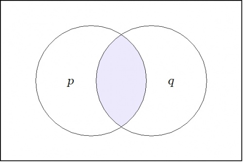
For example, consider the logical conjunction \(pq : X \to \mathbb{B}\!\) that is shown in the following venn diagram:
|
| \(\text{Conjunction}~ pq : X \to \mathbb{B}\!\) |
Each of the operators \(\mathrm{E}, \mathrm{D} : X^\circ \to \mathrm{E}X^\circ\!\) takes us from considering propositions \(f : X \to \mathbb{B},\!\) here viewed as scalar fields over \(X,\!\) to considering the corresponding differential fields over \(X,\!\) analogous to what are usually called vector fields over \(X.\!\)
The structure of these differential fields can be described this way. With each point of \(X\!\) there is associated an object of the following type: a proposition about changes in \(X,\!\) that is, a proposition \(g : \mathrm{d}X \to \mathbb{B}.\!\) In this frame of reference, if \({X^\circ}\!\) is the universe that is generated by the set of coordinate propositions \(\{ p, q \},\!\) then \(\mathrm{d}X^\circ\!\) is the differential universe that is generated by the set of differential propositions \(\{ \mathrm{d}p, \mathrm{d}q \}.\!\) These differential propositions may be interpreted as indicating \({}^{\backprime\backprime} \text{change in}\, p \, {}^{\prime\prime}\!\) and \({}^{\backprime\backprime} \text{change in}\, q \, {}^{\prime\prime},\!\) respectively.
A differential operator \(\mathrm{W},\!\) of the first order class that we have been considering, takes a proposition \(f : X \to \mathbb{B}\!\) and gives back a differential proposition \(\mathrm{W}f : \mathrm{E}X \to \mathbb{B}.\!\) In the field view, we see the proposition \(f : X \to \mathbb{B}\!\) as a scalar field and we see the differential proposition \(\mathrm{W}f : \mathrm{E}X \to \mathbb{B}\!\) as a vector field, specifically, a field of propositions about contemplated changes in \(X.\!\)
The field of changes produced by \(\mathrm{E}\!\) on \(pq\!\) is shown in the next venn diagram:
The differential field \(\mathrm{E}(pq)\!\) specifies the changes that need to be made from each point of \(X\!\) in order to reach one of the models of the proposition \(pq,\!\) that is, in order to satisfy the proposition \(pq.\!\)
The field of changes produced by \(\mathrm{D}\!\) on \(pq\!\) is shown in the following venn diagram:
The differential field \(\mathrm{D}(pq)\!\) specifies the changes that need to be made from each point of \(X\!\) in order to feel a change in the felt value of the field \(pq.\!\)
Proposition and Tacit Extension
Now that we've introduced the field picture as an aid to thinking about propositions and their analytic series, a very pleasing way of picturing the relationships among a proposition \(f : X \to \mathbb{B},\!\) its enlargement or shift map \(\mathrm{E}f : \mathrm{E}X \to \mathbb{B},\!\) and its difference map \(\mathrm{D}f : \mathrm{E}X \to \mathbb{B}\!\) can now be drawn.
To illustrate this possibility, let's return to the differential analysis of the conjunctive proposition \(f(p, q) = pq,\!\) giving the development a slightly different twist at the appropriate point.
The next venn diagram shows once again the proposition \(pq,\!\) which we now view as a scalar field — analogous to a potential hill in physics, but in logic tantamount to a potential plateau — where the shaded region indicates an elevation of 1 and the unshaded region indicates an elevation of 0.

|
| \(\text{Proposition}~ pq : X \to \mathbb{B}\!\) |
Given a proposition \(f : X \to \mathbb{B},\!\) the tacit extension of \(f\!\) to \(\mathrm{E}X\!\) is denoted \(\boldsymbol\varepsilon f : \mathrm{E}X \to \mathbb{B}~\!\) and defined by the equation \(\boldsymbol\varepsilon f = f,\!\) so it's really just the same proposition residing in a bigger universe. Tacit extensions formalize the intuitive idea that a function on a particular set of variables can be extended to a function on a superset of those variables in such a way that the new function obeys the same constraints on the old variables, with a "don't care" condition on the new variables.
The tacit extension of the scalar field \(pq : X \to \mathbb{B}\!\) to the differential field \(\boldsymbol\varepsilon (pq) : \mathrm{E}X \to \mathbb{B}\!\) is shown in the following venn diagram:
Enlargement and Difference Maps
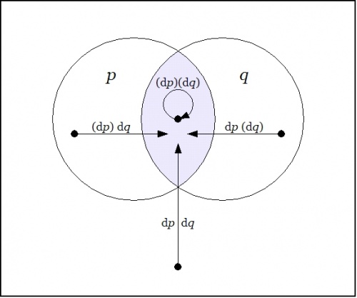
Continuing with the example \(pq : X \to \mathbb{B},\!\) the next venn diagram shows the enlargement or shift map \(\mathrm{E}(pq) : \mathrm{E}X \to \mathbb{B}\!\) in the same style of differential field picture that we drew for the tacit extension \(\boldsymbol\varepsilon (pq) : \mathrm{E}X \to \mathbb{B}.\!\)
A very important conceptual transition has just occurred here, almost tacitly, as it were. Generally speaking, having a set of mathematical objects of compatible types, in this case the two differential fields \(\boldsymbol\varepsilon f\!\) and \(\mathrm{E}f,\!\) both of the type \(\mathrm{E}X \to \mathbb{B},\!\) is very useful, because it allows us to consider these fields as integral mathematical objects that can be operated on and combined in the ways that we usually associate with algebras.
In this case one notices that the tacit extension \(\boldsymbol\varepsilon f\!\) and the enlargement \(\mathrm{E}f\!\) are in a certain sense dual to each other. The tacit extension \(\boldsymbol\varepsilon f\!\) indicates all the arrows out of the region where \(f\!\) is true and the enlargement \(\mathrm{E}f\!\) indicates all the arrows into the region where \(f\!\) is true. The only arc they have in common is the no-change loop \(\texttt{(} \mathrm{d}p \texttt{)(} \mathrm{d}q \texttt{)}\!\) at \(pq.\!\) If we add the two sets of arcs in mod 2 fashion then the loop of multiplicity 2 zeroes out, leaving the 6 arrows of \(\mathrm{D}(pq) = \boldsymbol\varepsilon(pq) + \mathrm{E}(pq)\!\) that are illustrated below:
Tangent and Remainder Maps
If we follow the classical line that singles out linear functions as ideals of simplicity, then we may complete the analytic series of the proposition \(f = pq : X \to \mathbb{B}\!\) in the following way.
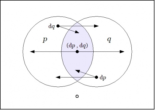
The next venn diagram shows the differential proposition \(\mathrm{d}f = \mathrm{d}(pq) : \mathrm{E}X \to \mathbb{B}\!\) that we get by extracting the cell-wise linear approximation to the difference map \(\mathrm{D}f = \mathrm{D}(pq) : \mathrm{E}X \to \mathbb{B}.\!\) This is the logical analogue of what would ordinarily be called the differential of \(pq,\!\) but since I've been attaching the adjective differential to just about everything in sight, the distinction tends to be lost. For the time being, I'll resort to using the alternative name tangent map for \(\mathrm{d}f.\!\)
|
| \(\text{Tangent Map}~ \mathrm{d}(pq) : \mathrm{E}X \to \mathbb{B}\!\) |
Just to be clear about what's being indicated here, it's a visual way of summarizing the following data:
|
\(\begin{array}{rcccccc} \mathrm{d}(pq) & = & p & \cdot & q & \cdot & \texttt{(} \mathrm{d}p \texttt{,} \mathrm{d}q \texttt{)} \\[4pt] & + & p & \cdot & \texttt{(} q \texttt{)} & \cdot & \mathrm{d}q \\[4pt] & + & \texttt{(} p \texttt{)} & \cdot & q & \cdot & \mathrm{d}p \\[4pt] & + & \texttt{(} p \texttt{)} & \cdot & \texttt{(} q \texttt{)} & \cdot & 0 \end{array}\!\) |
To understand the extended interpretations, that is, the conjunctions of basic and differential features that are being indicated here, it may help to note the following equivalences:
|
\(\begin{matrix} \texttt{(} \mathrm{d}p \texttt{,} \mathrm{d}q \texttt{)} & = & \texttt{~} \mathrm{d}p \texttt{~} \texttt{(} \mathrm{d}q \texttt{)} & + & \texttt{(} \mathrm{d}p \texttt{)} \texttt{~} \mathrm{d}q \texttt{~} \\[4pt] dp & = & \texttt{~} \mathrm{d}p \texttt{~} \texttt{~} \mathrm{d}q \texttt{~} & + & \texttt{~} \mathrm{d}p \texttt{~} \texttt{(} \mathrm{d}q \texttt{)} \\[4pt] \mathrm{d}q & = & \texttt{~} \mathrm{d}p \texttt{~} \texttt{~} \mathrm{d}q \texttt{~} & + & \texttt{(} \mathrm{d}p \texttt{)} \texttt{~} \mathrm{d}q \texttt{~} \end{matrix}\!\) |
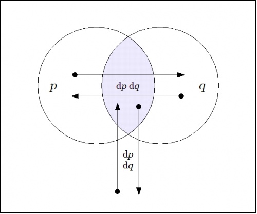
Capping the series that analyzes the proposition \(pq\!\) in terms of succeeding orders of linear propositions, the final venn diagram in this series shows the remainder map \(\mathrm{r}(pq) : \mathrm{E}X \to \mathbb{B},\!\) that happens to be linear in pairs of variables.
|
| \(\text{Remainder Map}~ \mathrm{r}(pq) : \mathrm{E}X \to \mathbb{B}\!\) |
Reading the arrows off the map produces the following data:
|
\(\begin{array}{rcccccc} \mathrm{r}(pq) & = & p & \cdot & q & \cdot & \mathrm{d}p ~ \mathrm{d}q \\[4pt] & + & p & \cdot & \texttt{(} q \texttt{)} & \cdot & \mathrm{d}p ~ \mathrm{d}q \\[4pt] & + & \texttt{(} p \texttt{)} & \cdot & q & \cdot & \mathrm{d}p ~ \mathrm{d}q \\[4pt] & + & \texttt{(} p \texttt{)} & \cdot & \texttt{(} q \texttt{)} & \cdot & \mathrm{d}p ~ \mathrm{d}q \end{array}\!\) |
In short, \(\mathrm{r}(pq)\!\) is a constant field, having the value \(\mathrm{d}p~\mathrm{d}q\!\) at each cell.
Least Action Operators
We have been contemplating functions of the type \(f : X \to \mathbb{B}\!\) and studying the action of the operators \(\mathrm{E}\!\) and \(\mathrm{D}\!\) on this family. These functions, that we may identify for our present aims with propositions, inasmuch as they capture their abstract forms, are logical analogues of scalar potential fields. These are the sorts of fields that are so picturesquely presented in elementary calculus and physics textbooks by images of snow-covered hills and parties of skiers who trek down their slopes like least action heroes. The analogous scene in propositional logic presents us with forms more reminiscent of plateaunic idylls, being all plains at one of two levels, the mesas of verity and falsity, as it were, with nary a niche to inhabit between them, restricting our options for a sporting gradient of downhill dynamics to just one of two: standing still on level ground or falling off a bluff.
We are still working well within the logical analogue of the classical finite difference calculus, taking in the novelties that the logical transmutation of familiar elements is able to bring to light. Soon we will take up several different notions of approximation relationships that may be seen to organize the space of propositions, and these will allow us to define several different forms of differential analysis applying to propositions. In time we will find reason to consider more general types of maps, having concrete types of the form \(X_1 \times \ldots \times X_k \to Y_1 \times \ldots \times Y_n\!\) and abstract types \(\mathbb{B}^k \to \mathbb{B}^n.\!\) We will think of these mappings as transforming universes of discourse into themselves or into others, in short, as transformations of discourse.
Before we continue with this intinerary, however, I would like to highlight another sort of differential aspect that concerns the boundary operator or the marked connective that serves as one of the two basic connectives in the cactus language for zeroth order logic.
For example, consider the proposition \(f\!\) of concrete type \(f : P \times Q \times R \to \mathbb{B}\!\) and abstract type \(f : \mathbb{B}^3 \to \mathbb{B}\!\) that is written \(\texttt{(} p, q, r \texttt{)}\!\) in cactus syntax. Taken as an assertion in what Peirce called the existential interpretation, the proposition \(\texttt{(} p, q, r \texttt{)}\!\) says that just one of \(p, q, r\!\) is false. It is instructive to consider this assertion in relation to the logical conjunction \(pqr\!\) of the same propositions. A venn diagram of \(\texttt{(} p, q, r \texttt{)}\!\) looks like this:

|
In relation to the center cell indicated by the conjunction \(pqr,\!\) the region indicated by \(\texttt{(} p, q, r \texttt{)}\!\) is comprised of the adjacent or bordering cells. Thus they are the cells that are just across the boundary of the center cell, reached as if by way of Leibniz's minimal changes from the point of origin, in this case, \(pqr.~\!\)
More generally speaking, in a \(k\!\)-dimensional universe of discourse that is based on the alphabet of features \(\mathcal{X} = \{ x_1, \ldots, x_k \},\!\) the same form of boundary relationship is manifested for any cell of origin that one chooses to indicate. One way to indicate a cell is by forming a logical conjunction of positive and negative basis features, that is, by constructing an expression of the form \(e_1 \cdot \ldots \cdot e_k,\!\) where \(e_j = x_j ~\text{or}~ e_j = \texttt{(} x_j \texttt{)},\!\) for \(j = 1 ~\text{to}~ k.\!\) The proposition \(\texttt{(} e_1, \ldots, e_k \texttt{)}\!\) indicates the disjunctive region consisting of the cells that are just next door to \(e_1 \cdot \ldots \cdot e_k.\!\)
Goal-Oriented Systems
I want to continue developing the basic tools of differential logic, which arose from exploring the connections between dynamics and logic, but I also wanted to give some hint of the applications that have motivated this work all along. One of these applications is to cybernetic systems, whether we see these systems as agents or cultures, individuals or species, organisms or organizations.
A cybernetic system has goals and actions for reaching them. It has a state space \(X,\!\) giving us all of the states that the system can be in, plus it has a goal space \(G \subseteq X,\!\) the set of states that the system “likes” to be in, in other words, the distinguished subset of possible states where the system is regarded as living, surviving, or thriving, depending on the type of goal that one has in mind for the system in question. As for actions, there is to begin with the full set \(\mathcal{T}\!\) of all possible actions, each of which is a transformation of the form \(T : X \to X,\!\) but a given cybernetic system will most likely have but a subset of these actions available to it at any given time. And even if we begin by thinking of actions in very general and very global terms, as arbitrarily complex transformations acting on the whole state space \(X,\!\) we quickly find a need to analyze and approximate them in terms of simple transformations acting locally. The preferred measure of “simplicity” will of course vary from one paradigm of research to another.
A generic enough picture at this stage of the game, and one that will remind us of these fundamental features of the cybernetic system even as things get far more complex, is afforded by Figure 23.
o---------------------------------------------------------------------o | | | X | | o-------------------o | | / \ | | / \ | | / \ | | / \ | | / \ | | / \ | | / \ | | o G o | | | | | | | | | | | | | | | o<---------T---------o | | | | | | | | | | | | | | o o | | \ / | | \ / | | \ / | | \ / | | \ / | | \ / | | \ / | | o-------------------o | | | | | o---------------------------------------------------------------------o Figure 23. Elements of a Cybernetic System |
Further Reading
A more detailed presentation of Differential Logic can be found here:
Document History
Differential Logic • Ontology List 2002
- http://web.archive.org/web/20140406040004/http://suo.ieee.org/ontology/msg04040.html
- http://web.archive.org/web/20110612001949/http://suo.ieee.org/ontology/msg04041.html
- http://web.archive.org/web/20110612010502/http://suo.ieee.org/ontology/msg04045.html
- http://web.archive.org/web/20110612005212/http://suo.ieee.org/ontology/msg04046.html
- http://web.archive.org/web/20110612001954/http://suo.ieee.org/ontology/msg04047.html
- http://web.archive.org/web/20110612010620/http://suo.ieee.org/ontology/msg04048.html
- http://web.archive.org/web/20110612010550/http://suo.ieee.org/ontology/msg04052.html
- http://web.archive.org/web/20110612010724/http://suo.ieee.org/ontology/msg04054.html
- http://web.archive.org/web/20110612000847/http://suo.ieee.org/ontology/msg04055.html
- http://web.archive.org/web/20110612001959/http://suo.ieee.org/ontology/msg04067.html
- http://web.archive.org/web/20110612010507/http://suo.ieee.org/ontology/msg04068.html
- http://web.archive.org/web/20110612002014/http://suo.ieee.org/ontology/msg04069.html
- http://web.archive.org/web/20110612010701/http://suo.ieee.org/ontology/msg04070.html
- http://web.archive.org/web/20110612003540/http://suo.ieee.org/ontology/msg04072.html
- http://web.archive.org/web/20110612005229/http://suo.ieee.org/ontology/msg04073.html
- http://web.archive.org/web/20110610153117/http://suo.ieee.org/ontology/msg04074.html
- http://web.archive.org/web/20110612010555/http://suo.ieee.org/ontology/msg04077.html
- http://web.archive.org/web/20110612001918/http://suo.ieee.org/ontology/msg04079.html
- http://web.archive.org/web/20110612005244/http://suo.ieee.org/ontology/msg04080.html
- http://web.archive.org/web/20110612005249/http://suo.ieee.org/ontology/msg04268.html
- http://web.archive.org/web/20110612010626/http://suo.ieee.org/ontology/msg04269.html
- http://web.archive.org/web/20110612000853/http://suo.ieee.org/ontology/msg04272.html
- http://web.archive.org/web/20110612010514/http://suo.ieee.org/ontology/msg04273.html
- http://web.archive.org/web/20110612002235/http://suo.ieee.org/ontology/msg04290.html
Dynamics And Logic • Inquiry List 2004
- http://stderr.org/pipermail/inquiry/2004-May/thread.html#1400
- http://stderr.org/pipermail/inquiry/2004-July/thread.html#1685
- http://stderr.org/pipermail/inquiry/2004-May/001400.html
- http://stderr.org/pipermail/inquiry/2004-May/001401.html
- http://stderr.org/pipermail/inquiry/2004-May/001402.html
- http://stderr.org/pipermail/inquiry/2004-May/001403.html
- http://stderr.org/pipermail/inquiry/2004-May/001404.html
- http://stderr.org/pipermail/inquiry/2004-May/001405.html
- http://stderr.org/pipermail/inquiry/2004-May/001406.html
- http://stderr.org/pipermail/inquiry/2004-May/001407.html
- http://stderr.org/pipermail/inquiry/2004-May/001408.html
- http://stderr.org/pipermail/inquiry/2004-May/001410.html
- http://stderr.org/pipermail/inquiry/2004-May/001411.html
- http://stderr.org/pipermail/inquiry/2004-May/001412.html
- http://stderr.org/pipermail/inquiry/2004-May/001413.html
- http://stderr.org/pipermail/inquiry/2004-May/001415.html
- http://stderr.org/pipermail/inquiry/2004-May/001416.html
- http://stderr.org/pipermail/inquiry/2004-May/001418.html
- http://stderr.org/pipermail/inquiry/2004-May/001419.html
- http://stderr.org/pipermail/inquiry/2004-May/001420.html
- http://stderr.org/pipermail/inquiry/2004-May/001421.html
- http://stderr.org/pipermail/inquiry/2004-May/001422.html
- http://stderr.org/pipermail/inquiry/2004-May/001423.html
- http://stderr.org/pipermail/inquiry/2004-May/001424.html
- http://stderr.org/pipermail/inquiry/2004-July/001685.html
- http://stderr.org/pipermail/inquiry/2004-July/001686.html
- http://stderr.org/pipermail/inquiry/2004-July/001687.html
- http://stderr.org/pipermail/inquiry/2004-July/001688.html
Dynamics And Logic • NKS Forum 2004
- http://forum.wolframscience.com/archive/topic/420.html
- http://forum.wolframscience.com/printthread.php?threadid=420
- http://forum.wolframscience.com/showthread.php?threadid=420
- http://forum.wolframscience.com/showthread.php?postid=1282#post1282
- http://forum.wolframscience.com/showthread.php?postid=1285#post1285
- http://forum.wolframscience.com/showthread.php?postid=1289#post1289
- http://forum.wolframscience.com/showthread.php?postid=1292#post1292
- http://forum.wolframscience.com/showthread.php?postid=1293#post1293
- http://forum.wolframscience.com/showthread.php?postid=1294#post1294
- http://forum.wolframscience.com/showthread.php?postid=1296#post1296
- http://forum.wolframscience.com/showthread.php?postid=1299#post1299
- http://forum.wolframscience.com/showthread.php?postid=1301#post1301
- http://forum.wolframscience.com/showthread.php?postid=1304#post1304
- http://forum.wolframscience.com/showthread.php?postid=1307#post1307
- http://forum.wolframscience.com/showthread.php?postid=1309#post1309
- http://forum.wolframscience.com/showthread.php?postid=1311#post1311
- http://forum.wolframscience.com/showthread.php?postid=1314#post1314
- http://forum.wolframscience.com/showthread.php?postid=1315#post1315
- http://forum.wolframscience.com/showthread.php?postid=1318#post1318
- http://forum.wolframscience.com/showthread.php?postid=1321#post1321
- http://forum.wolframscience.com/showthread.php?postid=1323#post1323
- http://forum.wolframscience.com/showthread.php?postid=1326#post1326
- http://forum.wolframscience.com/showthread.php?postid=1327#post1327
- http://forum.wolframscience.com/showthread.php?postid=1330#post1330
- http://forum.wolframscience.com/showthread.php?postid=1331#post1331
- http://forum.wolframscience.com/showthread.php?postid=1598#post1598
- http://forum.wolframscience.com/showthread.php?postid=1601#post1601
- http://forum.wolframscience.com/showthread.php?postid=1602#post1602
- http://forum.wolframscience.com/showthread.php?postid=1603#post1603
- Artificial Intelligence
- Boolean Algebra
- Boolean Functions
- Charles Sanders Peirce
- Combinatorics
- Computational Complexity
- Computer Science
- Cybernetics
- Differential Logic
- Equational Reasoning
- Formal Languages
- Formal Systems
- Graph Theory
- Inquiry
- Inquiry Driven Systems
- Knowledge Representation
- Logic
- Logical Graphs
- Mathematics
- Philosophy
- Propositional Calculus
- Semiotics
- Visualization


